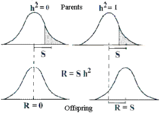
Selection response (R) equals the heritability multiplied by the difference in selection (S). The change is seen in the offspring

The term additive variance refers to the variance of breeding values (VA). (In some of the next chapters the symbol sigma2 is used synonymous with the variance.) Section 6.2 showed how the breeding value for each genotype in a locus could be estimated. When the genotype values are known, the additive variance for the locus can also be calculated. If independence occur between the loci, which have additive effect on a trait, then the joint additive variance will be the sum of variances from each locus. For individuals in a population the joint additive variance cannot be calculated directly, since the breeding value of the individuals is not known. It is not possible for all individuals to have the infinite number of offspring, which are required when the definition of breeding value is used. But VA can be calculated indirectly, as shown later in this chapter.
The phenotypic variance (VP), on the other hand, can always be calculated using the phenotypic values of the individuals in the population.
The heritability (h2) or the degree of heritability for a trait is defined as VA/VP. The heritability can vary between 0 and 1, since the additive variance is only part of the phenotypic variance.
Even though the additive variance cannot be directly estimated, the heritability can be estimated on the basis of the similarity between related individuals, which is measured either by a correlation or a regression. For instance, the regression of offspring on one of the parents. The heritability is estimated as the ratio of the calculated correlation coefficient and the coefficient of relationship. Which means that the maximum expected correlation between parent and offspring is 0.5. If the correlation coefficient is higher, it means that the similarity is caused by other factors besides the genetic.
The best method for estimating
the heritability is
the use of the correlation between half sibs, since they normally have only
genes in common. Full sibs, on the other hand, often have a maternal environment in
common too, which causes the litter
mates to be even more alike, and have more in common than genes. In such cases the heritability would be overestimated.
The parent-offspring correlation is seldom used in practise, since this method
needs data from two generations, often with different environment. It can also
be a problem if both parent and offspring live in the same environment.
Estimation of the variance component, caused by common environment for full sibs, can be carried out by comparing the estimated correlation based on respectively half and full sibs. The correlation between full sibs should be twice the one for half sibs. Often it is higher, the reason for this is that the full sibs have a common environment. This component is assigned the symbol c2, c for 'common environment'. The relative phenotypic variance has a genetic part (h2), a common environmental part (c2), and a third part. This remaining part of the variance is caused by random environmental effects, and gets the symbol e2. The random environmental part is for most traits the largest part of the phenotypic variance. Below is shown a table of the defined parameters.
Additive variance              VA
Phenotypic variance            VP
Heritability             	 h2
Common environment		 c2
Random environment	       e2
Half sib correlation      (1/4)h2
Full sib correlation      (1/2)h2 + c2
| Figure 6.3. Selection response (R) equals the heritability multiplied by the difference in selection (S). The change is seen in the offspring |
 |
Historically, the heritability has another interpretation. By selecting animals (shades area in Figure 6.3), which deviate from the mean value, the average of the next generation will change. The change is proportional to the difference in selection and the heritability following the formula:
R = h2*S
The selection response (R) equals the heritability multiplied by the selection difference (S). The heritability is 0, if the trait remains constant by selection, and it is 1, if the changes are equal to the selection difference, see Figure 6.3.