7.2 Estimating animal model breeding values
Other scripts can handle inbreeding, relationship, calculating the inverse
and estimating animal model breeding values. It will perform well up to 2000 observations and might be even more.
It has been made for solving smaller scientific problems and for educational purposes. It is worth to note that the numeration
of the animals is free as long as the oldest appear first. Link example
... Input aera .... ....Output area ....
The estimating the animal model breeding values, use the Evaluate botton after having put your data in the input area. You
can correct for any number of class variables
or continued variables in any combinations.
For class variables the fist class is excluded for not having
a degree of freedom as the mean value always is calculated.
Zero is treated as missing value so if zero is a part of the observation set a constant should be added.
The first 3 columns in the dataset shall contain animal, sire and dam - all other columns can be used freely. Link example
The first data line specify the parameters as follows - referring to first example below as well as in general
1.  1 specify (sigmaE/sigmaA)2  which in this case equals h2 = .50

2.  0 printing the solutions
    1 printing the solutions and the accuracy squared, for smaller number of data (pc-time problems)
    2 printing the triangualrization inclusive dependent var - last line the solutions
    3 printing the rearranged input with classes from zero to n-1 and dependent variable as the final.
    4 printing the equations inclusive the dependent var.
    5 printing all types of output

3.  0 normal model
    1 model with inbreeding - for smaller number of data (more roundings and pc-time problems)

4.- 0 exclude the trait from the analyses
    1 specify a continued variable where the last one is the dependent trait
   -1 specify the dependent trait if not the last trait -  which is then interchanged with the last variable
    2 specify a class variable
    3 specify a class variable but with all classes included (this can not be solved)
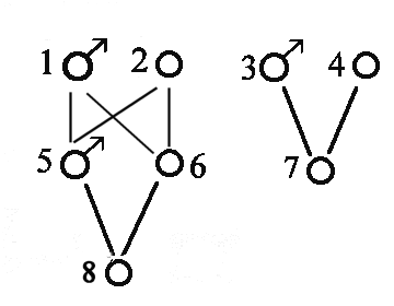
Example of estimating animal model breeding values for 8 animals, where the input file contains:
Animal Sire Dam, where 0 means unknown, one fixed factor, two continued vars. and the trait litter size
- except first line which specify the parameters explained above.
Put the data below in
the input window
followed by a return stroke


1 0 0 2 1 1  1
1 0 0 3 2 0  10
2 0 0 2 3 1   9
3 0 0 1 4 0   8
4 0 0 2 1 1   7
5 1 2 1 5 1   9
6 1 2 1 6 0  10
7 3 4 2 4 1   8
8 5 6 3 6 1  11
| Genealogical diagram
 |
 Resulting in


Animal model solutions

 1.0000	 0.1955
 2.0000	 0.4287
 3.0000	-0.3799
 4.0000	-0.2443
 5.0000	 0.3420
 6.0000	 0.3582
 7.0000	-0.4206
 8.0000	 0.2903
 0.0000	 6.9749	mean value
 2.0000	 0.5183	class  there is no degree of freedom for class 1
 3.0000	 1.8716	class
 0.0000	 0.4191	regression 1
 0.0000	-0.5322	regression 2
|
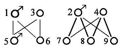
In the referred theory by Poul Jensen the first example on growth rate in young pigs can not be solved as the class year is given for all animals as follows.
But the system will nullify the first year and it is then converted to a regression giving 4.3883 gram extra the second year.
The heritability is set to 0.33.
2 0 0 2 1
1 0 0 0 0
2 0 0 1 225
3 0 0 1 220
4 0 0 1 255
5 1 3 2 250
6 1 3 2 198
7 2 4 2 245
8 2 4 2 260
9 2 4 2 235
|
Genealogical diagram
 |
Animal model solutions

animal   estimate

 1.0000	-3.1844
 2.0000	-0.3009
 3.0000	-6.2135
 4.0000	 9.6990
 5.0000	-1.0912
 6.0000	-11.4912
 7.0000	 5.4271
 8.0000	 8.4271
 9.0000	 3.4271
 0.0000	 232.2718
 0.0000	 4.3883
|
In case some of the parents are inbred the estimates will not be the same. In the following
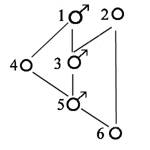
small example solutions are made with (parameter 3 set to 1) and without inbreeding. Example 2.1 from RA Mrode
'linear models for estimating breeding values, CABI Publishing'.
The heritability is set to 0.33.
2 0 1 1
1 0 0 15
2 0 0 19
3 1 2 7
4 1 0 13
5 4 3 22
6 5 2 10
|
Genealogical diagram
 |
Animal model solutions

not accounting for inbreeding

 1.0000	-0.3699
 2.0000	 0.1725
 3.0000	-1.0988
 4.0000	 0.1110
 5.0000	 0.7084
 6.0000	-0.5484
0.0000 14.5041 |
Animal model solutions

accounting for inbreeding

 1.0000	-0.3665
 2.0000	 0.1689
 3.0000	-1.0983
 4.0000	 0.1131
 5.0000	 0.7070
 6.0000	-0.4987
 0.0000	 14.4957
|
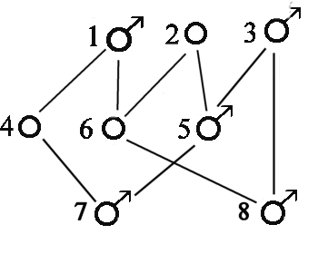
Estimating of the accuracy squared for the estimate; example 3.1 RA Mrode.
The heritability is set to 0.33.
2 1 0 2 1
1 0 0 0 0
2 0 0 0 0
3 0 0 0 0
4 1 0 1 4.5
5 3 2 2 2.9
6 1 2 2 3.9
7 4 5 1 3.5
8 3 6 1 5.0
|
Genealogical diagram
 |
Relationship matrix
1.00 0.00 0.00 0.00 0.50 0.50 0.00 0.00 0.00 0.00
0.00 1.00 0.00 0.00 0.00 0.00 0.50 0.50 0.50 0.00
0.00 0.00 1.00 0.00 0.50 0.50 0.00 0.00 0.00 0.00
0.00 0.00 0.00 1.00 0.00 0.00 0.50 0.50 0.50 0.00
0.50 0.00 0.50 0.00 1.00 0.50 0.00 0.00 0.00 0.00
0.50 0.00 0.50 0.00 0.50 1.00 0.00 0.00 0.00 0.00
0.00 0.50 0.00 0.50 0.00 0.00 1.00 0.50 0.50 0.00
0.00 0.50 0.00 0.50 0.00 0.00 0.50 1.00 0.50 0.00
0.00 0.50 0.00 0.50 0.00 0.00 0.50 0.50 1.00 0.00
0.00 0.00 0.00 0.00 0.00 0.00 0.00 0.00 0.00 1.00 |
The inverse Matrix
 2.00  0.00 1.00  0.00 -1.00 -1.00  0.00  0.00  0.00 0.00
 0.00  2.50 0.00  1.50 0.00   0.00 -1.00 -1.00 -1.00 0.00
1.00   0.00 2.00  0.00 -1.00 -1.00  0.00  0.00  0.00 0.00
 0.00  1.50 0.00  2.50 0.00   0.00 -1.00 -1.00 -1.00 0.00
-1.00  0.00 -1.00 0.00 2.00   0.00  0.00  0.00  0.00 0.00
-1.00  0.00 -1.00 0.00 0.00   2.00  0.00  0.00  0.00 0.00
 0.00 -1.00 0.00 -1.00 0.00   0.00  0.00  0.00  0.00 0.00
 0.00 -1.00 0.00 -1.00 0.00   0.00  0.00  2.00  0.00 0.00
 0.00 -1.00 0.00 -1.00 0.00   0.00  0.00  0.00  2.00 0.00
0.00 0.00 0.00 0.00 0.00 0.00 0.00 0.00 0.00 1.00 |
Larger example solutions for y, note that there is free numbering of the animals as long as the oldest occur first,
sex 2 has a 5.6002 units lower performance.
animal sire  dam  y  sex trait2

2 0 0 -1 1 2
1 0 0 0 0 0
2 0 0 0 0 0
3 0 0 0 0 0
4 0 0 0 0 0
5 0 0 0 0 0
6 0 0 0 0 0
7  0  0  93   2 2
8  1  2  78   1 2
9  1  2  63   1 3
10 1  3  91   1 3
11 1  3  70   2 3
12 1  3  100   2 2
13 1  4  102   1 4
14 1  5  119   1 5
15 1  5  121   2 4
16 1  6  93   2 6
17 1  6  81   2 4
18 1  6  82   2 3
19 14 17 78   2 2
20 14 17 88   1 5
21 14 17 85   2 6
22 14 7  91   2 5
23 14 7  113   1 7
24 14 7  118   2 5
25 14 15 91   2 4
26 14 15 83   2 2
27 14 15 102   1 4
128 14 12 87   2 5
29 14 12 83   1 3
30 14 12 86   1 3
31 14 16 106   2 4
32 14 16 90   1 5
33 14 16 57   2 3
34 23 25 82   1 2
35 23 25 84   1 1
36 23 25 77   2 3
37 23 22 83   2 2
38 23 128 95   1 5
39 23 128 68   2 4
40 23 31 116   1 6
41 23 31 112   1 7
42 23 31 88   2 5
43 23 24 121   1 4
44 23 24 98   1 4
45 23 24 86   1 4
|
Animal model solutions

The first variable contains numbers
of animal (mean) classes and regressions
and the second the estimate

 1.0000	-1.4325
 2.0000	-4.4927
 3.0000	 3.1002
 4.0000	 0.4142
 5.0000	 2.9162
 6.0000	-3.3706
 7.0000	 2.8651
 8.0000	-4.7612
 9.0000	-5.6569
 10.0000	 2.9802
 11.0000	-0.0996
 12.0000	 2.7212
 13.0000	-0.0949
 14.0000	-0.4850
 15.0000	 4.8850
 16.0000	-3.7721
 17.0000	-6.5152
 18.0000	-0.2880
 19.0000	-4.0711
 20.0000	-5.4854
 21.0000	-5.5097
 22.0000	-0.0535
 23.0000	-1.6506
 24.0000	 5.2497
 25.0000	 0.6864
 26.0000	 1.4889
 27.0000	 2.0724
 128.0000	-3.1481
 29.0000	 1.6076
 30.0000	 2.2076
 31.0000	 0.8187
 32.0000	-3.9882
 33.0000	-5.0696
 34.0000	-1.9767
 35.0000	-0.4821
 36.0000	 0.2475
 37.0000	-0.9527
 38.0000	-3.2048
 39.0000	-7.2870
 40.0000	 2.0375
 41.0000	-0.6642
 42.0000	-1.8980
 43.0000	 5.5520
 44.0000	 0.9520
 45.0000	-1.4479
 0.0000	 90.0823
 2.0000	 5.4732
 3.0000	-5.0481
 4.0000	 15.9558
 5.0000	 16.9446
 6.0000	 19.6661
 7.0000	 29.1753
 0.0000	-5.6002
|
The theory has been given by late Poul Jensen;
Back to theory 3 of animal model and back to theory 4 of animal model;
See also Erling Strandbergs notes
Back to the other programs
